Building in-house libraries: Python
The purpose of this section is to demonstrate how to build financial models using the Python functional programming paradigm. It is not to derive or implement models.
Thus we focus on two “toy” models - deterministic interest rates and 1-factor Gaussian short rate with constant coefficients.
Models
We consider models for the future evolution of discount factors. We restrict our implementation to the case when today’s interest rate curve is flat - the same rate for all (bond/deposit) maturities.
(In an actual analytics library, today’s rates input would be a curve - list of rates or discount factors and maturities, maybe along with an interpolation method.)
The simple discounting “model” (not really a model) assumes today’s rates stay the same in the future. Thus the discount factors are given by
(1)
where
is today’s spot interest rate,
is the valuation time (today -
, future
), and
is the maturity.
The Linear Gaussian model is
(2)
where
(3)
(4)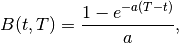
and
is the spot rate volatility and
is the spot rate mean reversion speed.
We can write down the price of any (interest rates) instrument in terms of discount factors. For example, the price of a coupon paying bond is
(5)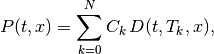
where  are the coupon amounts (
 the principal),
 the coupon dates, and
  the discount factors,
given by either (1) or (2).
(
the discount factors,
given by either (1) or (2).
(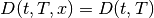 in (1))
The point is that we do just that in the implementation: Pass the functions calculating the discount factors to the (model agnostic) function that calculates the price of the coupon paying bond.
Similarly, any other (interest rates) model that can be plugged in (5). Likewise, other financial instruments (that can be written in terms of discount factors) can be priced in a similar way.
Implementation
Interest rates module - proof of concept
- LibPythonExample.intRates.cpnBondPrice(t, Tlist, Clist, x, discFactFun)[source]
This function implements (5). Tlist: -
, Clist - , equal length.- Usage:
- discFactFun = lambda t, T, x: discFactorDeterministic(t, T, r)
- or
- discFactFun = lambda t, T, x: discFactorLinearGaussian(t, T, r, x, a, v)
- Then
- P = cpnBondPrice(t, Tlist, Clist, x, disFactFun)

Tests
from LibPythonExample import intRates as intRates
t = 0.0
T = 2.0
x = 0.0
r = 0.02
a = 0.01
v = 0.03
fid = open('intRatesOut1.txt', 'w')
fid.write('Discount factors coincide for t=0, x=0:\n')
fid.write('Simple discounting: ' + str(intRates.discFactorDeterministic(t, T, r)) + '\n')
fid.write('Linear Gaussian:    ' + str(intRates.discFactorLinearGaussian(t, T, r, x, a, v))+ '\n')
t = 0.5
fid.write('\nDiscount factors are different for t>0, x=0:\n')
fid.write('Simple discounting: ' + str(intRates.discFactorDeterministic(t, T, r))+ '\n')
fid.write('Linear Gaussian:    ' + str(intRates.discFactorLinearGaussian(t, T, r, x, a, v))+ '\n')
x = 0.02
fid.write('\nOr for x>0 \n')
fid.write('Simple discounting: ' + str(intRates.discFactorDeterministic(t, T, r))+ '\n')
fid.write('Linear Gaussian:    ' + str(intRates.discFactorLinearGaussian(t, T, r, x, a, v))+ '\n')
###
fid.write('\nPrice of coupon paying bond for t>0, x>0:\n')
Tlist = [1.0, 2.0, 3.0, 4.0]
Clist = [0.05, 0.05, 0.05, 1.05]
simpleDiscFun = lambda t0, T0, x0: intRates.discFactorDeterministic(t0, T0, r)
linGaussFun   = lambda t0, T0, x0: intRates.discFactorLinearGaussian(t0, T0, r, x0, a, v)
fid.write('Simple discounting: ' + str(intRates.cpnBondPrice(t, Tlist, Clist, x, simpleDiscFun))+ '\n')
fid.write('Linear Gaussian:    ' + str(intRates.cpnBondPrice(t, Tlist, Clist, x, linGaussFun))+ '\n')
fid.close()
Discount factors coincide for t=0, x=0:
Simple discounting: 0.9607894391523232
Linear Gaussian:    0.9607894391523232

Discount factors are different for t>0, x=0:
Simple discounting: 0.9607894391523232
Linear Gaussian:    0.9710890479916172

Or for x>0
Simple discounting: 0.9607894391523232
Linear Gaussian:    0.9426000342280054

Price of coupon paying bond for t>0, x>0:
Simple discounting: 4.163442212442078
Linear Gaussian:    3.94614421159158